Two diseases in LCT-based SECIR-type model
The LCT-SECIR-2-DISEASES model is an extension of the model with one disease. The model is ODE-based and uses the Linear Chain Trick to allow for more general Erlang distributed stay times in each compartment instead of just exponentially distributed stay times induced by basic ODE-based models. With the SECIR structure the model is particularly suited for pathogens with pre- or asymptomatic infection states and when severe or critical states are possible. For the two diseases or variants of one disease \(a\) and \(b\) the model assumes no co-infection, a certain independence in the sense that prior infection with one disease does not affect the infection with the other disease (e.g. probability to get infected, time spend in each state, chances of recovery etc.), and perfect immunity after recovery for both diseases.
- There are two possibilities for a susceptible individual (since we assume no co-infection):
Get infected with disease a, then (if not dead) get infected with disease b
Get infected with disease b, then (if not dead) get infected with disease a
Each infection is simulated using a LCT-SECIR model. The states are labeled according to infection (first or second) and disease (\(a\) or \(b\)), so the full model is given by the combination of infections \(1a\), \(2a\), \(1b\), and \(2b\).
Below is a visualization of the infection states split into LCT-states and transitions without a stratification according to sociodemographic groups.
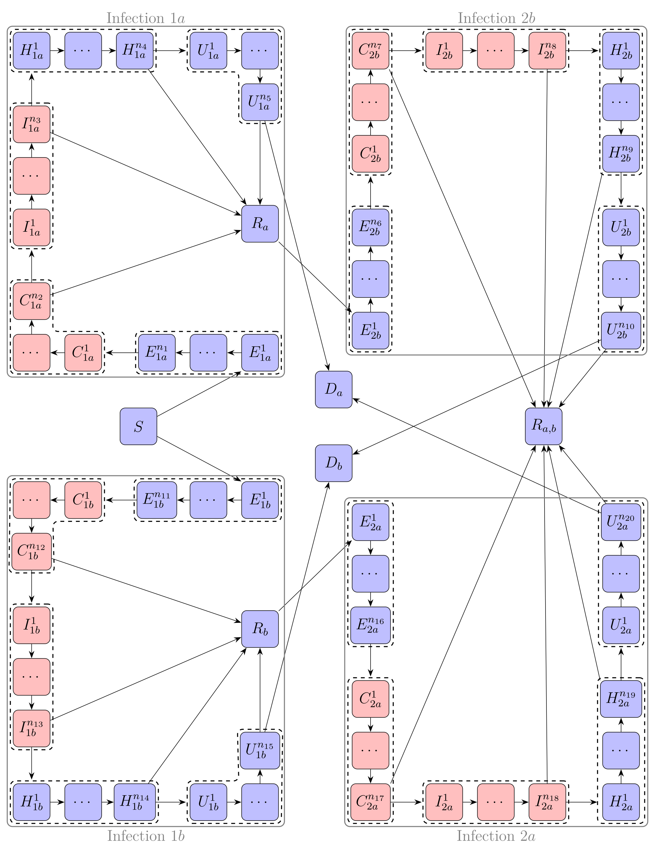
With infection states for \(i \in \{1,2\}, x \in \{a,b\}\):
Letter |
SECIR-State |
In the code |
|---|---|---|
S |
Susceptible |
Susceptible |
E |
Exposed |
Exposed_ix |
C |
Carrier |
InfectedNoSymptoms_ix |
I |
Infected |
InfectedSymptoms_ix |
H |
Hospitalized |
InfectedSevere_ix |
U |
in Intensive Care Unit |
InfectedCritical_ix |
R |
Recovered |
Recovered_x, Recoverd_ab |
D |
Dead |
Dead_x |
The compartments \(C, I\) are infectious (red), the other compartments are considered to be not infectious (blue), due to extensive isolation of the hospitalized individuals.
Infection States
The model contains the following list of InfectionStates:
`Susceptible`

`Exposed_1a`
`InfectedNoSymptoms_1a`
`InfectedSymptoms_1a`
`InfectedSevere_1a`
`InfectedCritical_1a`

`Recovered_a`
`Dead_a`

`Exposed_2a`
`InfectedNoSymptoms_2a`
`InfectedSymptoms_2a`
`InfectedSevere_2a`
`InfectedCritical_2a`

`Exposed_1b`
`InfectedNoSymptoms_1b`
`InfectedSymptoms_1b`
`InfectedSevere_1b`
`InfectedCritical_1b`

`Recovered_b`
`Dead_b`

`Exposed_2b`
`InfectedNoSymptoms_2b`
`InfectedSymptoms_2b`
`InfectedSevere_2b`
`InfectedCritical_2b`

`Recovered_ab`
It is possible to include subcompartments for the states E, C, I, H, and U, so compartments Exposed_1a, Exposed_2a, Exposed_1b, Exposed_2b, InfectedNoSymptoms_1a, InfectedNoSymptoms_2a, InfectedNoSymptoms_1b, InfectedNoSymptoms_2b, InfectedSymptoms_1a , InfectedSymptoms_2a, InfectedSymptoms_1b , InfectedSymptoms_2b, InfectedSevere_1a, InfectedSevere_2a , InfectedSevere_1b , InfectedSevere_2b, InfectedCritical_1a, InfectedCritical_2a, InfectedCritical_1b, and InfectedCritical_2b.
The number of subcompartments can be set individually for each compartment.
Sociodemographic Stratification
In the LCT-SECIR-2D model, the population can be stratified by one sociodemographic dimension. This dimension is denoted Group. It can be used for age groups as well as for other interpretations. Different age groups can have different numbers of subcompartments.
Parameters
The model implements the following parameters:
Mathematical variable |
C++ variable name |
Description |
|---|---|---|
\(\phi\) |
|
Average number of contacts for person per day, for multiple age groups this is a matrix. |
\(\rho_a\) |
|
Transmission risk for people located in the susceptible compartments for disease \(a\). |
\(\rho_b\) |
|
Transmission risk for people located in the susceptible compartments for disease \(b\). |
\(\xi_{I_{NS}, a}\) |
|
Proportion of nonsymptomatically infected people who are not isolated for disease \(a\). |
\(\xi_{I_{NS}, b}\) |
|
Proportion of nonsymptomatically infected people who are not isolated for disease \(b\). |
\(\xi_{I_{Sy}, a}\) |
|
Proportion of infected people with symptoms who are not isolated for disease \(a\). |
\(\xi_{I_{Sy}, b}\) |
|
Proportion of infected people with symptoms who are not isolated for disease \(b\). |
\(N\) |
|
Total population. |
\(n_{E,1a}\) |
Defined in |
Number of subcompartments of the Exposed_1a compartment. |
\(n_{E,2a}\) |
Defined in |
Number of subcompartments of the Exposed_2a compartment. |
\(n_{E,1b}\) |
Defined in |
Number of subcompartments of the Exposed_1b compartment. |
\(n_{E,2b}\) |
Defined in |
Number of subcompartments of the Exposed_2b compartment. |
\(n_{NS,1a}\) |
Defined in |
Number of subcompartments of the InfectedNoSymptoms_1a compartment. |
\(n_{NS,2a}\) |
Defined in |
Number of subcompartments of the InfectedNoSymptoms_2a compartment. |
\(n_{NS,1b}\) |
Defined in |
Number of subcompartments of the InfectedNoSymptoms_1b compartment. |
\(n_{NS,2b}\) |
Defined in |
Number of subcompartments of the InfectedNoSymptoms_2b compartment. |
\(n_{Sy,1a}\) |
Defined in |
Number of subcompartments of the InfectedSymptoms_1a compartment. |
\(n_{Sy,2a}\) |
Defined in |
Number of subcompartments of the InfectedSymptoms_2a compartment. |
\(n_{Sy,1b}\) |
Defined in |
Number of subcompartments of the InfectedSymptoms_1b compartment. |
\(n_{Sy,2b}\) |
Defined in |
Number of subcompartments of the InfectedSymptoms_2b compartment. |
\(n_{Sev,1a}\) |
Defined in |
Number of subcompartments of the InfectedSevere_1a compartment. |
\(n_{Sev,2a}\) |
Defined in |
Number of subcompartments of the InfectedSevere_2a compartment. |
\(n_{Sev,1b}\) |
Defined in |
Number of subcompartments of the InfectedSevere_1b compartment. |
\(n_{Sev,2b}\) |
Defined in |
Number of subcompartments of the InfectedSevere_2b compartment. |
\(n_{Cr,1a}\) |
Defined in |
Number of subcompartments of the InfectedCritical_1a compartment. |
\(n_{Cr,2a}\) |
Defined in |
Number of subcompartments of the InfectedCritical_2a compartment. |
\(n_{Cr,1b}\) |
Defined in |
Number of subcompartments of the InfectedCritical_1b compartment. |
\(n_{Cr,2b}\) |
Defined in |
Number of subcompartments of the InfectedCritical_2b compartment. |
\(T_{E,a}\) |
|
Average time in days an individual stays in the Exposed_1a or Exposed_2a compartment. |
\(T_{E,b}\) |
|
Average time in days an individual stays in the Exposed_1b or Exposed_2b compartment. |
\(T_{I_{NS},a}\) |
|
Average time in days an individual stays in the InfectedNoSymptomsa_1a or InfectedNoSymptoms_2a compartment. |
\(T_{I_{NS},b}\) |
|
Average time in days an individual stays in the InfectedNoSymptomsa_1b or InfectedNoSymptoms_2b compartment. |
\(T_{I_{Sy},a}\) |
|
Average time in days an individual stays in the InfectedSymptoms_1a or InfectedSymptoms_2a compartment. |
\(T_{I_{Sy},b}\) |
|
Average time in days an individual stays in the InfectedSymptoms_1b or InfectedSymptoms_2b compartment. |
\(T_{I_{Sev},a}\) |
|
Average time in days an individual stays in the InfectedSevere_1a or InfectedSevere_2a compartment. |
\(T_{I_{Sev},b}\) |
|
Average time in days an individual stays in the InfectedSevere_1b or InfectedSevere_2b compartment. |
\(T_{I_{Cr},a}\) |
|
Average time in days an individual stays in the InfectedCritical_1a or InfectedCritical_2a compartment. |
\(T_{I_{Cr},b}\) |
|
Average time in days an individual stays in the InfectedCritical_1b or InfectedCritical_2b compartment. |
\(\mu_{I_{NS},a}^{R}\) |
|
Probability of transition from compartment InfectedNoSymptoms_1a to Recovered_a or from InfectedNoSymptoms_2a to Recovered_ab. |
\(\mu_{I_{NS},b}^{R}\) |
|
Probability of transition from compartment InfectedNoSymptoms_1b to Recovered_b or from InfectedNoSymptoms_2b to Recovered_ab. |
\(\mu_{I_{Sy},a}^{I_{Sev}}\) |
|
Probability of transition from compartment InfectedSymptoms_1a to InfectedSevere_1a or from InfectedSymptoms_2a to InfectedSevere_2a. |
\(\mu_{I_{Sy},b}^{I_{Sev}}\) |
|
Probability of transition from compartment InfectedSymptoms_1b to InfectedSevere_1b or from InfectedSymptoms_2b to InfectedSevere_2b. |
\(\mu_{I_{Sev},a}^{I_{Cr}}\) |
|
Probability of transition from compartment InfectedSevere_1a to InfectedCritical_1a or from InfectedSevere_2a to InfectedCritical_2a. |
\(\mu_{I_{Sev},b}^{I_{Cr}}\) |
|
Probability of transition from compartment InfectedSevere_1b to InfectedCritical_1b or from InfectedSevere_2b to InfectedCritical_2b. |
\(\mu_{I_{Cr},a}^{D}\) |
|
Probability of dying when in compartment InfectedCritical_1a or InfectedCritical_2a. |
\(\mu_{I_{Cr},b}^{D}\) |
|
Probability of dying when in compartment InfectedCritical_1b or InfectedCritical_2b. |
Initial conditions
To initialize the model, we start by defining the number of subcompartments for every compartment and constructing the model with it.
constexpr size_t NumExposed_1a = 1, NumInfectedNoSymptoms_1a = 1, NumInfectedSymptoms_1a = 1,
                 NumInfectedSevere_1a = 1, NumInfectedCritical_1a = 1, NumExposed_2a = 1,
                 NumInfectedNoSymptoms_2a = 1, NumInfectedSymptoms_2a = 1, NumInfectedSevere_2a = 1,
                 NumInfectedCritical_2a = 1, NumExposed_1b = 1, NumInfectedNoSymptoms_1b = 1,
                 NumInfectedSymptoms_1b = 1, NumInfectedSevere_1b = 1, NumInfectedCritical_1b = 1,
                 NumExposed_2b = 1, NumInfectedNoSymptoms_2b = 1, NumInfectedSymptoms_2b = 1,
                 NumInfectedSevere_2b = 1, NumInfectedCritical_2b = 1;
using InfState = mio::lsecir2d::InfectionState;
using LctState = mio::LctInfectionState<
    InfState, 1, NumExposed_1a, NumInfectedNoSymptoms_1a, NumInfectedSymptoms_1a, NumInfectedSevere_1a,
    NumInfectedCritical_1a, 1, 1, NumExposed_2a, NumInfectedNoSymptoms_2a, NumInfectedSymptoms_2a,
    NumInfectedSevere_2a, NumInfectedCritical_2a, NumExposed_1b, NumInfectedNoSymptoms_1b, NumInfectedSymptoms_1b,
    NumInfectedSevere_1b, NumInfectedCritical_1b, 1, 1, NumExposed_2b, NumInfectedNoSymptoms_2b,
    NumInfectedSymptoms_2b, NumInfectedSevere_2b, NumInfectedCritical_2b, 1>;
using Model = mio::lsecir2d::Model<LctState>;
Model model;
For the simulation, we need initial values for all (sub)compartments. If we do not set the initial values manually, these are set to \(0\) by default.
We start with constructing a vector initial_populations that we will pass on to the model. It contains vectors for each compartment,
that contains a vector with initial values for the respective subcompartments.
std::vector<std::vector<ScalarType>> initial_populations = {
    {200},  {0, 0},  {30, 10, 0}, {0, 0, 0}, {0, 0, 0}, {0, 0},     {0},       {0},       {0},
    {0, 0}, {10, 0}, {0, 0},      {0},       {10, 0},   {30, 0, 0}, {0, 0, 0}, {0, 0, 0}, {0, 0},
    {0},    {0},     {100},       {0, 0},    {0, 0},    {0, 0},     {0},       {0}};
We assert that the vector has the correct size by checking that the number of InfectionStates and the numbers of subcompartments are correct.
if (initial_populations.size() != (size_t)InfState::Count) {
    mio::log_error("The number of vectors in initial_populations does not match the number of InfectionStates.");
    return 1;
}
if ((initial_populations[(size_t)InfState::Susceptible].size() !=
     LctState::get_num_subcompartments<InfState::Susceptible>()) ||
    (initial_populations[(size_t)InfState::Exposed_1a].size() != NumExposed_1a) ||
    (initial_populations[(size_t)InfState::InfectedNoSymptoms_1a].size() != NumInfectedNoSymptoms_1a) ||
    (initial_populations[(size_t)InfState::InfectedSymptoms_1a].size() != NumInfectedSymptoms_1a) ||
    (initial_populations[(size_t)InfState::InfectedSevere_1a].size() != NumInfectedSevere_1a) ||
    (initial_populations[(size_t)InfState::InfectedCritical_1a].size() != NumInfectedCritical_1a) ||
    (initial_populations[(size_t)InfState::Exposed_2a].size() != NumExposed_2a) ||
    (initial_populations[(size_t)InfState::InfectedNoSymptoms_2a].size() != NumInfectedNoSymptoms_2a) ||
    (initial_populations[(size_t)InfState::InfectedSymptoms_2a].size() != NumInfectedSymptoms_2a) ||
    (initial_populations[(size_t)InfState::InfectedSevere_2a].size() != NumInfectedSevere_2a) ||
    (initial_populations[(size_t)InfState::InfectedCritical_2a].size() != NumInfectedCritical_2a) ||
    (initial_populations[(size_t)InfState::Recovered_a].size() !=
     LctState::get_num_subcompartments<InfState::Recovered_a>()) ||
    (initial_populations[(size_t)InfState::Dead_a].size() !=
     LctState::get_num_subcompartments<InfState::Dead_a>()) ||
    (initial_populations[(size_t)InfState::Exposed_1b].size() != NumExposed_1b) ||
    (initial_populations[(size_t)InfState::InfectedNoSymptoms_1b].size() != NumInfectedNoSymptoms_1b) ||
    (initial_populations[(size_t)InfState::InfectedSymptoms_1b].size() != NumInfectedSymptoms_1b) ||
    (initial_populations[(size_t)InfState::InfectedSevere_1b].size() != NumInfectedSevere_1b) ||
    (initial_populations[(size_t)InfState::InfectedCritical_1b].size() != NumInfectedCritical_1b) ||
    (initial_populations[(size_t)InfState::Exposed_2b].size() != NumExposed_2b) ||
    (initial_populations[(size_t)InfState::InfectedNoSymptoms_2b].size() != NumInfectedNoSymptoms_2b) ||
    (initial_populations[(size_t)InfState::InfectedSymptoms_2b].size() != NumInfectedSymptoms_2b) ||
    (initial_populations[(size_t)InfState::InfectedSevere_2b].size() != NumInfectedSevere_2b) ||
    (initial_populations[(size_t)InfState::InfectedCritical_2b].size() != NumInfectedCritical_2b) ||
    (initial_populations[(size_t)InfState::Recovered_ab].size() !=
     LctState::get_num_subcompartments<InfState::Recovered_ab>())) {
        mio::log_error("The length of at least one vector in initial_populations does not match the related number of "
                      "subcompartments.");
        return 1;
    }
The initial populations in the model are set via:
std::vector<ScalarType> flat_initial_populations;
for (auto&& vec : initial_populations) {
    flat_initial_populations.insert(flat_initial_populations.end(), vec.begin(), vec.end());
}
for (size_t i = 0; i < LctState::Count; i++) {
    model.populations[i] = flat_initial_populations[i];
}
Nonpharmaceutical Interventions
In the LCT-SECIR-2D model, nonpharmaceutical interventions (NPIs) are implemented through dampings in the contact matrix. These dampings reduce the contact rates between different groups to simulate interventions.
Basic dampings can be added to the contact matrix as follows:
// Create a contact matrix with constant contact rate 10 (one age group).
mio::ContactMatrixGroup& contact_matrix = model.parameters.get<mio::lsecir2d::ContactPatterns>();
contact_matrix[0]                       = mio::ContactMatrix(Eigen::MatrixXd::Constant(1, 1, 10));

// From SimulationTime 5, the contact pattern is reduced to 30% of the initial value.
contact_matrix[0].add_damping(0.7, mio::SimulationTime(5.));
For age-resolved models, you can apply different dampings to different groups:
// Create a contact matrix with constant contact rate 10 between all age groups
contact_matrix[0] = mio::ContactMatrix(Eigen::MatrixXd::Constant(num_agegroups, num_agegroups, 10));

// Add a damping that reduces contacts within the same age group by 70% starting at day 5.
contact_matrix.add_damping(Eigen::VectorX<ScalarType>::Constant(num_agegroups, 0.7).asDiagonal(),
                         mio::SimulationTime(5.));
Simulation
We can simulate the model from \(t_0\) to \(t_{\max}\) with initial step size \(dt\) as follows:
ScalarType t0 = 0;
ScalarType tmax = 10;
ScalarType dt = 0.5;
mio::TimeSeries<ScalarType> result = mio::simulate<ScalarType, Model>(t0, tmax, dt, model);
Output
The simulation result is stratefied by subcompartments. The function calculate_compartments() aggregates the subcompartments by InfectionStates.
mio::TimeSeries<ScalarType> population_no_subcompartments = model.calculate_compartments(result);
You can access the data in the mio::TimeSeries object as follows:
// Get the number of time points.
auto num_points = static_cast<size_t>(result.get_num_time_points());

// Access data at a specific time point.
Eigen::VectorX value_at_time_i = result.get_value(i);
ScalarType time_i = result.get_time(i);

// Access the last time point.
Eigen::VectorX last_value = result.get_last_value();
ScalarType last_time = result.get_last_time();
You can print the simulation results as a formatted table:
// Print results to console with default formatting.
result.print_table();

// Print with custom column labels and width, and custom number of decimals.
results.print_table({"   S",   "   E1a", "   C1a", "   I1a", "   H1a", "   U1a", "   Ra",
                                  "   Da",  "   E2a", "   C2a", "   I2a", "   H2a", "   U2a", "   E1b",
                                  "   C1b", "   I1b", "   H1b", "   U1b", "   Rb",  "   Db",  "   E2b",
                                  "   C2b", "   I2b", "   H2b", "   U2b", "   Rab"},
                                 6, 2);
Additionally, you can export the results to a CSV file:
// Export results to CSV with default settings.
result.export_csv("simulation_results.csv");
Visualization
To visualize the results of a simulation, you can use the Python package m-plot and its documentation.
Examples
An example can be found at:
The code documentation for the model can be found at mio::lsecir2d .