ODE-based MSEIRS4 model (ODE)
The ODE-MSEIRS4 module models a pathogen with partial and waning immunity across multiple infection episodes, including a maternal immunity class. It is suited for pathogens with repeat infections and seasonality.
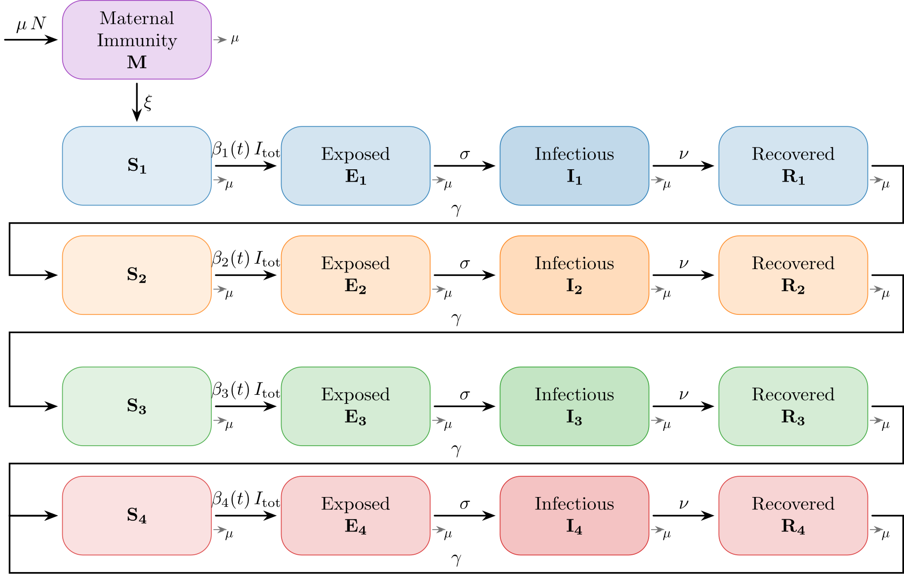
The infection states and the transitions are visualized in the following graph.
This implementation is designed for Respiratory Syncytial Virus (RSV) and is based on:
Weber A, Weber M, Milligan P. (2001). Modeling epidemics caused by respiratory syncytial virus (RSV). Mathematical Biosciences 172(2): 95–113. DOI:10.1016/S0025-5564(01)00066-9
Infection States
The model contains the following InfectionStates:
MaternalImmune (M)
S1, S2, S3, S4 (susceptible classes by infection history)
E1, E2, E3, E4 (exposed/latent for the k-th infection episode)
I1, I2, I3, I4 (infectious for the k-th infection episode)
R1, R2, R3, R4 (recovered following the k-th infection episode)
Meaning of indices 1–4
S1: fully susceptible after loss of maternal immunity (highest susceptibility; seasonal force β1(t)).
S2: susceptible after first infection (R1 → S2 via waning; reduced susceptibility; β2(t)=f2·β1(t)).
S3: susceptible after second infection (R2 → S3; β3(t)=f3·β1(t)).
S4: susceptible after ≥3 infections (R3 → S4 and R4 → S4; lowest susceptibility; β4(t)=f4·β1(t)).
The multipliers \(f_2, f_3, f_4\) are dimensionless susceptibility reductions for S2–S4. All infectious classes (I1..I4) contribute equally to transmission in the basic formulation.
Infection State Transitions
The model is implemented as a CompartmentalModel, which defines the derivative of the aggregated compartment values in time. The following transitions occur:
Births enter M and some enter S1
M → S1 (loss of maternal immunity)
S_k → E_k
E_k → I_k
I_k → R_k
R1 → S2, R2 → S3, R3 → S4 and R4 → S4 (waning immunity)
Natural deaths apply to all compartments
Seasonality
Time unit is days. Seasonality follows a yearly cosine:
Here, \(b_0\) is the base transmission rate (per day), \(b_1\in[0,1]\) the seasonal amplitude, and \(\varphi\) a phase (radians).
Parameters
The model implements the following parameters:
Mathematical symbol |
C++ parameter name |
Description |
|---|---|---|
\(b_0\) |
|
Base transmission rate (per day). |
\(b_1\) |
|
Seasonal amplitude. |
\(\varphi\) |
|
Phase of the cosine forcing (radians). |
\(\mu\) |
|
Natural birth/death rate (per day). |
\(\xi\) |
|
Rate of losing maternal immunity M→S1 (per day). |
\(\sigma\) |
|
Progression rate E→I (per day). |
\(\nu\) |
|
Recovery rate I→R (per day). |
\(\gamma\) |
|
Waning rate R→S stage (per day). |
\(f_2\) |
|
Susceptibility multiplier for S2. |
\(f_3\) |
|
Susceptibility multiplier for S3. |
\(f_4\) |
|
Susceptibility multiplier for S4. |
Initial conditions
Initial conditions are absolute counts in each InfectionState; totals may be set directly.
Example (see examples/ode_mseirs4.cpp) shows a complete initialization and simulation.
The code documentation for the model can be found at mio::omseirs4 .
Simulation
Run a standard simulation via:
double t0 = 0.0;     // days
double tmax = 3650;  // 10 years
double dt = 1.0;     // daily step
auto timeseries = mio::simulate(t0, tmax, dt, model);
Output
The output is a mio::TimeSeries of compartment sizes over time. Use print_table or export to CSV as needed.
Notes
Homogeneous mixing; no age/contact matrices in this variant.
All rates are per day.
As in the paper, the model keeps N approximately constant if births and deaths balance.
References
Weber A, Weber M, Milligan P. (2001). Modeling epidemics caused by respiratory syncytial virus (RSV). Mathematical Biosciences 172(2): 95–113. DOI:10.1016/S0025-5564(01)00066-9