ODE-based SEIRDB model

The ODE-SEIRDB module models and simulates Ebola-like dynamics with explicit dead and buried compartments using an ODE-based SEIR-type extension. It is suited for simple simulations with explicit death and burial handling. The model assumes perfect immunity after recovery

The infection states and the transitions are visualized in the following graph.

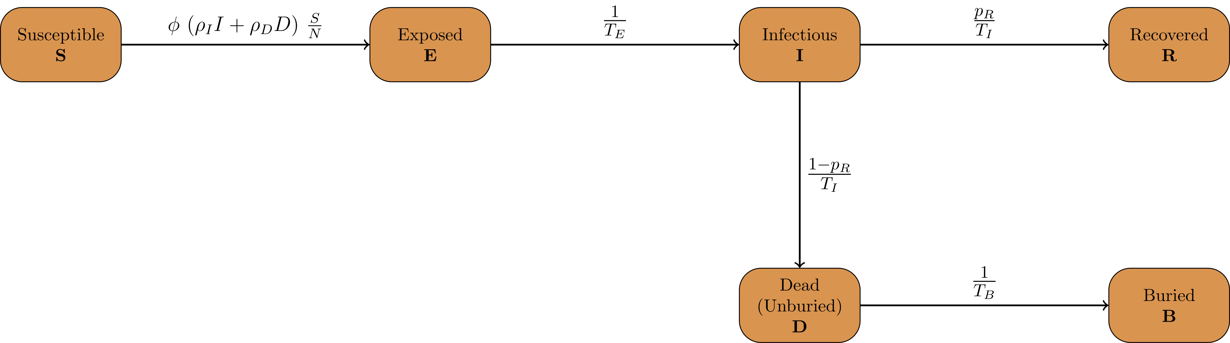
Infection States

The model contains the following list of InfectionStates:

`Susceptible`
`Exposed`
`Infected`
`Recovered`
`Dead`
`Buried`

Infection State Transitions

The ODE-SEIRDB model is implemented as a FlowModel, which defines the derivatives of each flow between compartments. This allows for explicit computation of new transmissions, infections, recoveries, deaths, and burials. Additionally, the aggregated compartment values can be computed with minimal overhead. The defined transitions FromState, ToState are:

`Susceptible,  Exposed`
`Exposed,      Infected`
`Infected,     Recovered`
`Infected,     Dead`
`Dead,         Buried`

Sociodemographic Stratification

In the ODE-SEIRDB model, the population can be stratified by one sociodemographic dimension. This dimension is denoted AgeGroup but can also be used for other interpretations. For stratifications with two or more dimensions, see Model Creation.

The number of age groups is specified in the model constructor and the model can be initialized with

mio::oseirdb::Model model(nb_groups)

Parameters

The model implements the following parameters:

Mathematical variable	C++ variable name	Description
\(\phi\)	`ContactPatterns`	Matrix of daily contact rates / number of daily contacts between different age groups.
\(\rho_I\)	`TransmissionProbabilityOnContact`	Transmission risk for people located in the Infected compartment.
\(\rho_D\)	`TransmissionProbabilityFromDead`	Transmission risk for people in the Dead-but-unburied compartment.
\(p_R\)	`ProbabilityToRecover`	Probability that an infected person recovers (vs. dies).
\(N\)	`populations.get_total()`	Total population.
\(T_{E}\)	`TimeExposed`	Time in days an individual stays in the Exposed compartment.
\(T_{I}\)	`TimeInfected`	Time in days an individual stays in the Infected compartment.
\(T_{B}\)	`TimeToBurial`	Time in days an individual stays in the Dead compartment before burial.

Initial Conditions

The initial conditions of the model are defined by the class Populations which defines the number of individuals in each sociodemographic group and InfectionState. Before running a simulation, you need to set the initial values for each compartment:

// Set total population size
model.populations.set_total(nb_total_t0);

// Set values for each InfectionState in the specific age group
model.populations[{mio::AgeGroup(0), mio::oseirdb::InfectionState::Exposed}] = nb_exp_t0;
model.populations[{mio::AgeGroup(0), mio::oseirdb::InfectionState::Infected}] = nb_inf_t0;
model.populations[{mio::AgeGroup(0), mio::oseirdb::InfectionState::Recovered}] = nb_rec_t0;
model.populations[{mio::AgeGroup(0), mio::oseirdb::InfectionState::Dead}]      = nb_dead_t0;
model.populations[{mio::AgeGroup(0), mio::oseirdb::InfectionState::Buried}]    = nb_buried_t0;


// Set the susceptible population as difference to ensure correct total population
model.populations.set_difference_from_total({mio::AgeGroup(0), mio::oseirdb::InfectionState::Susceptible}, nb_total_t0);

For age-resolved simulations, you need to set the initial conditions for each age group. Additionally, you can use set_difference_from_group_total to set the susceptible compartment as the difference between the total group size and all other compartments:

for(auto i = mio::AgeGroup(0); i < nb_groups; i++){
   model.populations[{i, mio::oseirdb::InfectionState::Exposed}] = 1/nb_groups * nb_exp_t0;
   model.populations[{i, mio::oseirdb::InfectionState::Infected}] = 1/nb_groups * nb_inf_t0;
   model.populations.set_difference_from_group_total({i, mio::oseirdb::InfectionState::Susceptible}, nb_total_t0);
}

Nonpharmaceutical Interventions

In the ODE-SEIRDB model, nonpharmaceutical interventions (NPIs) are implemented through dampings to the contact matrix. These dampings reduce the contact rates between different sociodemographic groups to simulate interventions.

Basic dampings can be added to the ContactPatterns as follows:

// Create a contact matrix with constant contact rates between all groups
mio::ContactMatrixGroup& contact_matrix = model.parameters.get<mio::oseirdb::ContactPatterns<double>>();
contact_matrix[0] = mio::ContactMatrix(Eigen::MatrixXd::Constant(1, 1, cont_freq));

// Add a damping that reduces contacts by 70% starting at day 30
contact_matrix[0].add_damping(0.7, mio::SimulationTime(30.));

For age-resolved models, you can apply different dampings to different age groups:

contact_matrix[0] = mio::ContactMatrix(Eigen::MatrixXd::Constant((size_t)nb_groups, (size_t)nb_groups, 1/nb_groups * cont_freq));

// Add a damping that reduces contacts within the same age group by 70% starting at day 30
contact_matrix.add_damping(Eigen::VectorX<ScalarType>::Constant((size_t)nb_groups, 0.7).asDiagonal(),
                         mio::SimulationTime(30.));

Simulation

The ODE-SEIRDB model offers two simulation functions:

simulate: Standard simulation that tracks the compartment sizes over time
simulate_flows: Extended simulation that additionally tracks the flows between compartments

Standard simulation:

double t0 = 0;       // Start time
double tmax = 50;    // End time
double dt = 0.1;     // Initial step size

// Run a standard simulation
mio::TimeSeries<double> result_sim = mio::oseirdb::simulate(t0, tmax, dt, model);

Flow simulation for tracking transitions between compartments:

// Run a flow simulation to additionally track transitions between compartments
auto result_flowsim = mio::oseirdb::simulate_flows(t0, tmax, dt, model);
// result_flowsim[0] contains compartment sizes, result_flowsim[1] contains flows

For both simulation types, you can also specify a custom integrator:

auto integrator = std::make_unique<mio::RKIntegratorCore>();
integrator->set_dt_min(0.3);
integrator->set_dt_max(1.0);
integrator->set_rel_tolerance(1e-4);
integrator->set_abs_tolerance(1e-1);

mio::TimeSeries<double> result_sim = mio::oseirdb::simulate(t0, tmax, dt, model, std::move(integrator));

Output

The output of the Simulation is a mio::TimeSeries containing the sizes of each compartment at each time point. For A standard simulation, you can access the results as follows:

// Get the number of time points
auto num_points = static_cast<size_t>(result_sim.get_num_time_points());

// Access data at specific time point
Eigen::VectorXd value_at_time_point_i = result_sim.get_value(i);
double time_i = result_sim.get_time(i);

// Access the last time point
Eigen::VectorXd last_value = result_sim.get_last_value();
double last_time = result_sim.get_last_time();

For flow simulations, the result consists of two mio::TimeSeries objects, one for compartment sizes and one for flows:

// Access compartment sizes
auto compartments = result_flowsim[0];

// Access flows between compartments
auto flows = result_flowsim[1];

You can print the simulation results as a formatted table via:

// Print results to console with default formatting
result_sim.print_table();

// Print with custom column labels
std::vector<std::string> labels = {"S", "E", "I", "R", "D", "B"};
result_sim.print_table(labels);

Additionally, you can export the results to a CSV file:

// Export results to CSV with default settings
result_sim.export_csv("simulation_results.csv");

Visualization

To visualize the results of a simulation, you can use the Python package m-plot and its documentation.

Examples

An example can be found at examples/ode_seirdb.cpp.

The code documentation for the model can be found at mio::oseirdb .