ODE-based SEIRV model

The ODE-SEIRV module extends the classic SEIR model by an explicit vaccinated layer (S^V, E^V, I^V, R^V) and targets seasonal influenza–type applications (cf. Weidemann et al. 2017). It is age-structured and uses a normalized contact matrix formulation with explicit seasonality. Immunity after recovery is assumed to last for the considered season. Also, there is no transition between the unvaccinated and vaccinated compartments during the simulation horizon (i.e., no vaccinations after season start).

The infection states and transitions are illustrated in the following figure.

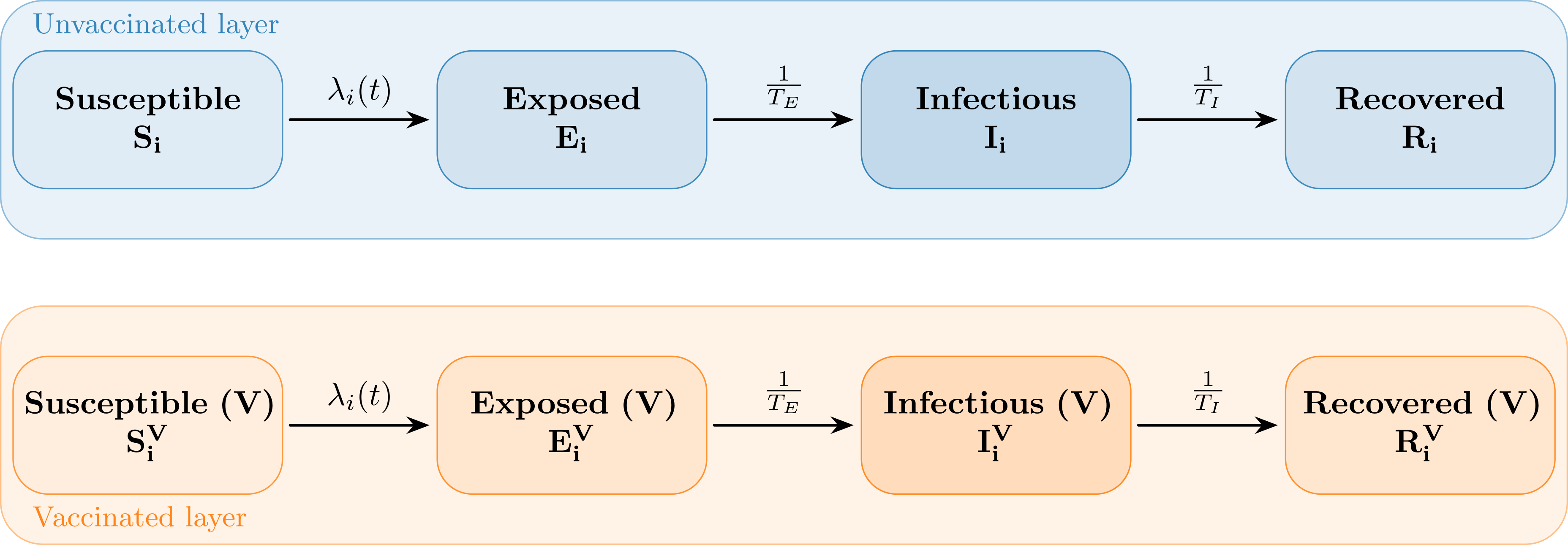
Infection States

The model contains the following InfectionStates:

`Susceptible`
`SusceptibleVaccinated`
`Exposed`
`ExposedVaccinated`
`Infected`
`InfectedVaccinated`
`Recovered`
`RecoveredVaccinated`

Infection State Transitions

The SEIRV model is implemented as a FlowModel. Thus, in each time step, the flows (new infections, progressions, recoveries) are computed explicitly in addition to compartment values. The defined transitions FromState, ToState are:

`Susceptible,           Exposed`
`SusceptibleVaccinated, ExposedVaccinated`
`Exposed,               Infected`
`ExposedVaccinated,     InfectedVaccinated`
`Infected,              Recovered`
`InfectedVaccinated,    RecoveredVaccinated`

Sociodemographic Stratification

The population can be stratified by one sociodemographic dimension denoted AgeGroup (can be interpreted more broadly). The number of age groups is specified in the constructor:

mio::oseirv::Model<double> model(num_agegroups);

For stratifications with two or more dimensions, see Model Creation.

Parameters

The model uses the following parameters (time unit: week):

Mathematical Symbol	C++ Name / Type	Description
\(R_e\)	`BaselineTransmissibility`	Baseline transmissibility (dimensionless); scales the normalized force of infection.
\(T_E\)	`TimeExposed`	Mean time (weeks) in the exposed compartment; progression E -> I occurs with rate \(1/T_E\).
\(T_I\)	`TimeInfected`	Mean infectious time (weeks); progression I -> R occurs with rate \(1/T_I\) and the force of infection scales with \(1/T_I\).
\(\delta\)	`SeasonalityAmplitude`	Amplitude of the seasonal modulation \(\exp(\delta\,\sin(2\pi(t/52 - t_z + t_s)))\).
\(t_z\)	`SeasonalityShiftPerSubtype`	Coarse (subtype-specific) seasonal phase shift.
\(t_s\)	`SeasonalityShiftPerSeason`	Fine seasonal phase adjustment per season.
\(\lambda_0\)	`OutsideFoI`	External (additive) force of infection, can seed infections.
\(\rho\)	`ClusteringExponent`	Clustering exponent on the infectious fraction.
\(m\)	`SickMixing`	Mixing weight for symptomatic (“sick”) contacts in the blended contact matrix.
\(C^{H}\)	`ContactPatternsHealthy`	Age-structured contact matrix (healthy). Can be time-dependent via damping.
\(C^{S}\)	`ContactPatternsSick`	Age-structured contact matrix (symptomatic), combined using \(m\).
\(\sigma_i\)	`CustomIndexArray`	Age-specific baseline susceptibility (pre-existing immunity modifier).
\(VC_i\)	`VaccineCoverage`	Vaccination coverage per age group at season start (share vaccinated).
\(VE_i\)	`VaccineEffectiveness`	Vaccine effectiveness (reducing effective susceptibility).
\(\phi_0\)	`SusceptibleFraction`	Fraction of the total population forming the effectively susceptible pool at \(t_0\).

Note: VaccineCoverage and VaccineEffectiveness are only used for initialization. Transitions presently apply identical hazards to vaccinated and unvaccinated susceptible compartments. Future extensions may introduce differential infection hazards.

Initial Conditions

Initial conditions are handled via the Populations class. Example for a single age group:

mio::oseirv::Model<double> model(1);
// Set total population in age group 0
model.populations.set_total(total0);

// Initialize vaccinated susceptibles (simple example)
double vc0 = 0.4; // vaccination coverage
model.populations[{mio::AgeGroup(0), mio::oseirv::InfectionState::SusceptibleVaccinated}] = vc0 * total0;
model.populations[{mio::AgeGroup(0), mio::oseirv::InfectionState::Infected}] = initial_infected;
model.populations[{mio::AgeGroup(0), mio::oseirv::InfectionState::Exposed}]  = initial_exposed;

// Other states (Recovered / RecoveredVaccinated) often 0 at season start

// Set remaining susceptibles as difference
model.populations.set_difference_from_total(
                {mio::AgeGroup(0), mio::oseirv::InfectionState::Susceptible}, total0);

For age-resolved simulations, repeat for each age group; set_difference_from_group_total ensures correct susceptible counts:

for (auto a = mio::AgeGroup(0); a < num_agegroups; ++a) {
                model.populations[{a, mio::oseirv::InfectionState::Exposed}]  = exposed0 / num_agegroups;
                model.populations[{a, mio::oseirv::InfectionState::Infected}] = infected0 / num_agegroups;
                model.populations[{a, mio::oseirv::InfectionState::SusceptibleVaccinated}] = vc[a.get()] * group_size[a.get()];
                model.populations.set_difference_from_group_total<mio::AgeGroup>(
                                {a, mio::oseirv::InfectionState::Susceptible}, group_size[a.get()]);
}

Simulation

Like other ODE models in MEmilio, the SEIRV model can be simulated with standard compartment output or with explicit flows. Once integrated with utility wrappers (analogous to oseir::simulate / simulate_flows) usage follows the same pattern. Example with a Runge–Kutta integrator:

double t0   = 0.0;  // start (weeks)
double tmax = 20.0; // end
double dt   = 0.1;  // initial step size

auto integrator = std::make_unique<mio::RKIntegratorCore>();
integrator->set_dt_min(0.01);
integrator->set_dt_max(0.5);
integrator->set_rel_tolerance(1e-4);
integrator->set_abs_tolerance(1e-6);

auto sim = mio::simulate(t0, tmax, dt, model, std::move(integrator));

Flow simulation (when explicit flows are required):

auto flowsim = mio::simulate_flows(t0, tmax, dt, model);
// flowsim[0] = compartment sizes, flowsim[1] = flows

Output

The result of a standard simulation is a mio::TimeSeries:

auto n_points = static_cast<size_t>(sim.get_num_time_points());
Eigen::VectorXd val_i = sim.get_value(i);
double time_i = sim.get_time(i);
auto last_val = sim.get_last_value();

Printing and CSV export:

sim.print_table();
std::vector<std::string> labels = {"S","S_V","E","E_V","I","I_V","R","R_V"};
sim.print_table(labels);
sim.export_csv("seirv_results.csv");

Contact Changes / Interventions

Time-dependent changes of contact patterns (holidays, interventions) can be modeled via dampings (add_damping) on ContactPatternsHealthy and/or ContactPatternsSick:

mio::ContactMatrixGroup<ScalarType>& cm_h = model.parameters.get<mio::oseirv::ContactPatternsHealthy<double>>();
mio::ContactMatrixGroup<ScalarType>& cm_s = model.parameters.get<mio::oseirv::ContactPatternsSick<double>>();
cm_h[0] = mio::ContactMatrix(Eigen::MatrixXd::Constant(num_agegroups, num_agegroups, base_contacts));
cm_s[0] = mio::ContactMatrix(Eigen::MatrixXd::Constant(num_agegroups, num_agegroups, base_contacts_sick));

// Reduce healthy contacts by 40% starting at week 5
cm_h[0].add_damping(0.6, mio::SimulationTime(5.0));

Visualization

For visualization you can use the Python package m-plot as in the other models.

Literature

Weidemann, F., Remschmidt, C., Buda, S. et al. Is the impact of childhood influenza vaccination less than expected: a transmission modelling study. BMC Infectious Diseases 17, 258 (2017). https://doi.org/10.1186/s12879-017-2344-6

The code documentation for the model can be found at mio::oseirv .